LARGE SCALE OPTIMIZATION | EFFICIENT FRONTIER | RETURN AND VARIANCE MODELS |

Return and Variance Models

Before starting, it is important to keep in mind that whatever technique is used to measure the performance of assets, the resulting model is essentially phenomenological, without no physical laws to support predictions. In that sense, simplicity and interpretability go a long way in producing a useful and effective model.

The models used for portfolio optimization by the Optimize API are expected return and variance asset models. See references [1-3] and this case study for details. In such models, an asset return is represented by two quantities: the expected return, $ \mu_i $, and its variance, $ \sigma_i^2 $, that is $$ \begin{aligned} \mu_{i} &= E \{ r_i \}, & \sigma_i^2 = c_{i,i} &= E \{ (r_i - \mu_i)^2 \}. \end{aligned} $$ With more than one asset, we add to the model the correlation between each asset, $$ c_{i,j} = E \{ (r_i - \mu_i) (r_j - \mu_j) \}. $$

The expected return and variance of a portfolio is then optimized by evaluating $$ \begin{aligned} \mu(\theta) &= \sum_{i} \theta_i \, \mu_i, & \sigma^2(\theta) &= \sum_{i, j} c_{i, j} \, \theta_i \, x_j, \end{aligned} $$ in which $ \theta_i $ is the asset's weight on the portfolio (more on portfolio weights and some not so obvious caveats below).

For a given portfolio, expected return and variance for each asset and their covariances can be estimated by the Models API. This note goes over some important aspects that need to be taken into account when estimating returns and variances and their use in portfolio optimization.

Historic Asset Prices

Expected returns and their variances are typically estimated from historic price series^[1]. As the number of parameters to be estimated grows with the square of the size of the number of assets in the portfolio, so does the demand on data and the uncertainty about those estimates.

In this case study, we highlight some difficulties involved in the estimation of expected returns and variances. From the choice of return series to use to the methodology employed to calculate the estimates, it is quite easy to get astray and end up with models that are not very representative.

To make the discussion concrete, we shall work with two particular assets: NVDA and TQQQ. Their adjusted^[2] price series, retrieved and calculated over the course of the last five years at the time of this note writing, October 2024, is shown in the plots below.

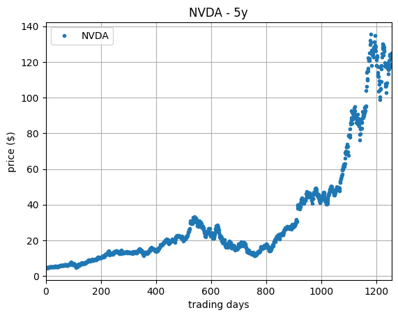
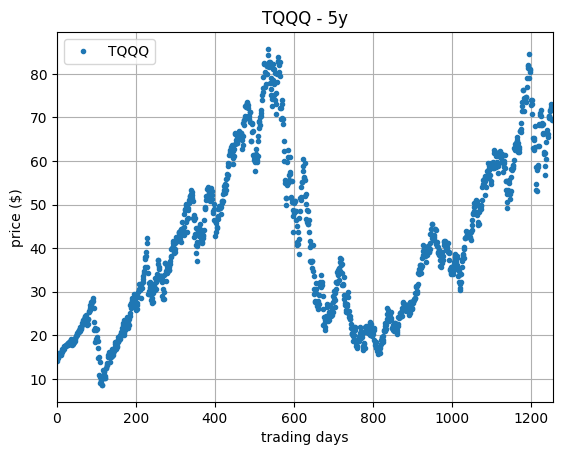
As so much has happened within the last five years, this is a very interesting period to study. As for singling out these two assets, NVDA seems an obvious choice given its recent incredible exponential growth, while TQQQ displays some interesting ups-and-downs.

Daily Returns

A naive approach to estimating the return of assets is to calculate the statistics of the daily returns. If $ p[k] $ denotes the price of an asset at day $ k $, then

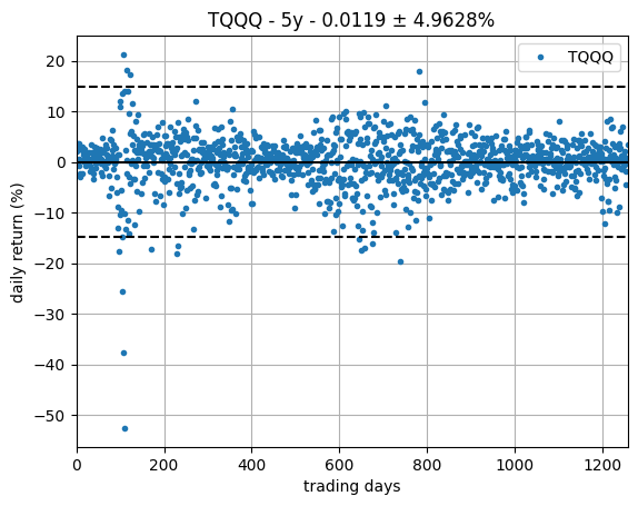
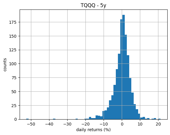
$$ r[k] = \frac{p[k] - p[k-1]}{p[k-1]} $$ is the corresponding daily return. For TQQQ, the corresponding series of daily returns is ploted on the right.

For each series of daily returns we calculate the sample mean ($ \hat{\mu} $) and sample standard deviation ($ \hat{\sigma} $). In the daily return plot, the solid line is the mean and the dashed lines are the corresponding 3-$ \sigma $ intervals.

Without putting much thought into it, notice that the estimated mean return is expected to be tiny when compared with the variance of the daily returns, which can make its estimation tricky. Before proceeding, we take a look at the histogram of the daily return series to assess how close to normal or at least symmetrically distributed it looks, as a way to support the use of the simple statistics above. The histogram, shown in the next plot, does not immediately raises suspicions.

If we substitute the daily return by its expected value, that is $ r[k] = \mu $, then we are implicitly assuming that $ p[k] $ evolves as $$ p[k] = (1 + \mu) \, p[k-1] $$ or, in other words, that the price evolution is the exponential $$ p[k] = (1 + \mu)^k \, p[0]. $$ Substituting $ \mu $ for the estimated sample mean $ \hat{\mu} $ and superimposing the resulting exponential to the price series we obtain the plot on the right, in which the predicted price estimated by the model is the orange solid curve.

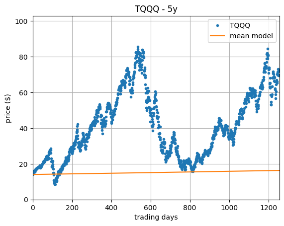
It is striking how the above estimate fails to match the original price behaviour. One may attempt to improve the model by looking at other statistics of the daily returns, for one example, the median. No matter how one tries to massage the series of daily returns into producing a return model which looks reasonable when compared with the evolution of the price, one will always find an asset for which the model quality is subpar. In order to obtain better models we need to work directly with prices.

Prices, Returns, and the Power of Log

Estimating returns based on simple aggregate statistics of the daily return series turned out not to be a good idea. For one thing, the mean or any other aggregate statistic of the daily returns do not take into account when that return happened. In fact, if one permutes the daily returns, one would still obtain the same aggregate statistics, but yet completely different price series.

It also happens that knowing how an asset performed on a particular day in the past is not very informative when it comes to assessing the asset's performance measured with respect to today's price. What an investor cares to know is how much one would have today if he or she had invested at a certain point in time. That is not the series of daily returns, but rather the series of compound returns as measured from any point in time until today. If we let $ p[n] $ denote the price of the asset today, then what we are after is the value of $ r_n[k] $ such that $$ p[n] = \left ( 1 + r_n[k] \right )^{n-k} p[k], \qquad k < n. $$ Due to the multiplicative nature of returns, it is easier to work with the logarithm of the prices, rather than with the prices. More specifically, it is better to work with the much simpler quantity $$ a[k] = \log(1 + r_n[k]) = \frac{\log p[k] - \log p[n]}{k - n}, \qquad k < n. $$

For more insight, one can rearrange the above equation into the form $$ \log p[k] = \log p[n] + a[k] \, (k - n) $$ which, for a constant $ a[k] = \mu_{a} $, can be identified with an equation of the form $$ y = y_n + \mu_{a} \, (x - x_n). $$ This is a line with slope $ \mu_{a} $ that passes through the point $ (x_n, y_n) $. Indeed, $ y = y_n $ when $ x = x_n $. In terms of the log-price,

$$ \underbrace{\log p[k]}_{y} = \underbrace{\log p[n]}_{y_n} + \mu_{a} \, (\underbrace{k - n}_{x - x_n}). $$

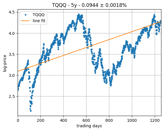
The above discussion provides a different perspective from which to estimate an asset's return: as the slope of the best fit line that goes by today's price in logarithmic scale.

Such an estimate can be obtained by performing a standard linear regression. The plot on the right show the result of such a fit for our favorite asset, TQQQ, which is much more sensible than the one obtained before from the statistics of the daily returns.

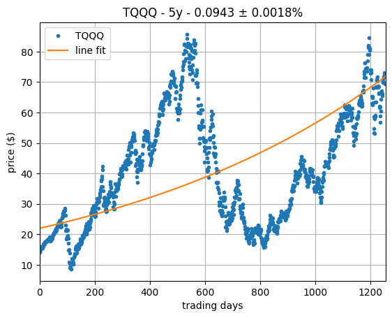
From logarithmic scale, we can convert back to linear scale in order to obtain the corresponding exponential model, shown in the plot on the right, which also looks very reasonable.

As a bonus, the linear fit interpretation comes with built-in estimates for the variance of the estimated slopes, which we can adopt as estimates for the asset return variance. One caveat here is that those estimates are obtained in logarithmic scale, and they need to be properly translated back into linear scale for use in portfolio optimization. In the same vein, it is not immediately clear how to proceed on estimating the correlation between assets, or to construct factor models^[3,4]. All of these details are taken care by the algorithms implemented in the Models API. In translating from logarithmic scale to linear and vice-versa, the algorithms in Models API employ the formalism of log-normal models [3, $ \S $16.7].

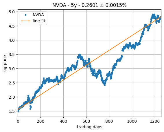
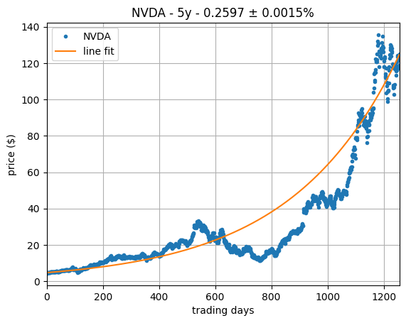
As a sanity check, we repeat the above exercise for a second asset, this time NVDA, which results in the logarithmic and exponential fits on the plots on the right, which shows even better results.

The Return of Portfolios

Having found a satisfactory ways in which to estimate returns and variances of individual assets, we now turn to the problem of using such models for optimizing portfolios. It is worth clearly stating our fairly modest goals. We are after two numbers, the elusive expected return and its variance, which represent the performance of the portfolio based on estimates of the returns and covariances of the individual assets in that portfolio.

Whereas one might be tempted to simply plugging in the estimated assets' return and covariance into the portfolio optimization model, it is important to pay attention to one missing ingredient: the investor's investment horizon. At a minimum, it is important to match the periodicity with which the estimates were calculated to the investor investment horizon. The expected daily return and variance might mean little for an investor who is not interested in trading daily! It is necessary to take into account the effects of long-term investing [3, $ \S $10].

Consider a portfolio with $ m $ assets. Over time, the portfolio is priced at $$ \pi[k] = \sum_{i = 1}^{m} x_i[k], $$ in which $ x_i[k] $ is the value of the $ i $th asset at day $ k $. If the number of shares of each asset in a portfolio is kept constant and equal to today's number of shares, then $$ x_i[k] = \frac{p_i[k]}{p_i[n]} x_i[n], \qquad \text{for all } i \text{ and } k, $$ in which $ p_i[k] $ is the price of each share of the $ i $th asset at day $ k $. In that case $$ \begin{aligned} \frac{\pi[k]}{\pi[n]} &= \sum_{i = 1}^{m} \theta_i \frac{p_i[k]}{p_i[n]}, \qquad \theta_i = \frac{x_i[n]}{\pi[n]} \geq 0, \quad \sum_{i = 1}^m \theta_i = 1. \end{aligned} $$ The $ \theta_i $'s are the portfolio weights. Clearly, it only makes sense to optimize portfolio weights if one also knows how long the investor is expected to keep the portfolio shares constant, that is if we know the investment horizon. Moreover, the impact of holding a portfolio constant is inexorable: in the long term, the portfolio becomes the asset with the highest return [3, $ \S $ 10]. How long is “long-term” depends heavily on the composition of the portfolio as well as the investment horizon, but the compounding of daily returns usually means that one month might be already long-term when it comes to returns and their covariances.

As with individual assets, it is better to evaluate the return of portfolios in the log-domain $$ \begin{aligned} \alpha[k] &= \frac{\log \pi[k] - \log \pi[n]}{k - n} = \frac{\log \sum_{i = 1}^{m} \theta_i \, (p_i[k]/p_i[n])}{k - n} = \frac{\log \sum_{i = 1}^{m} \theta_i \, e^{a_i[k] (k-n)}}{k - n}. \end{aligned} $$ Note that the portfolio return over time, $ \alpha[k] $, is never constant, even if the individual assets' returns, the $ a_i $'s, were constant, which is another way to state the impact of long-term holdings mentioned above. A better measure of the portfolio return over a given investment horizon, say a horizon of $ q $ days, is $$ \mu[n+q] = \sum_{i = 1}^{m} \theta_i \, \mu_i[n+q], \qquad \mu_i[n+q] = e^{q \, a_i[n+1]} - 1. $$

After the above discussion, it seems paramount that one adjusts the individual assets' expected return and variance before attempting to optimize a portfolio. It is for this reason that the models produced by the Models API, have their returns and covariances adjusted to match a given investment horizon.

That's enough for today. We shall continue discussing models here in future case studies.

Mauricio de Oliveira

References

Harry M. Markowitz, “Portfolio Selection”. Journal of Finance, 7(1): 77 - 91, 1952.
Edwin J. Elton and Martin J. Gruber, Modern Portfolio Theory and Investment Analysis. Fifth Edition, John Wiley and Sons, 1995.
Mark S. Joshi and Jane M. Paterson, Introduction to Mathematical Portfolio Theory. Cambridge University Press, 2013.

Notes

During optimization, investors might want to merge prospective or predictive models based on fundamentals or other considerations.
After compensating for splits and dividends.
Estimating all covariance parameters in large-scale portfolios is a tricky task. More often than not, optimal portfolios end up exploiting features of the covariance matrix that end up in the model via uncertainties in the estimation procedure. Factor models reduce the need to estimat all covariance parameters by structuring the returns as a function of a reduced set of factors, which can be thought of playing a proxy role for a diversified market portfolio. One such typical structure is in the form $$ C = C_\alpha + \beta \, C_f \, \beta^T. $$ In the above model, $ C_\alpha $ is usually a diagonal matrix, and the covariance matrix $ C_f $ is the covariance matrix of the factors. See the next note for more details in how those matrices are constructed.
Factor models are typically obtained by first establishing a relationship between the assets and the factors. For example, $$ r_i = \alpha_i + \sum_{k} \beta_{i,k} f_k + \epsilon_i $$ expresses a linear relationship between the return of the $ i $th asset and the factors $ f_k $'s. The coefficient $ \alpha_i $ represents the intrinsic or unsystematic portion of the returns, whereas the $ \beta_{i,j} $'s represent the systematic part. Here again, logarithms complicate things, and one needs to be careful in calculating model estimates.